
A fire pump hydraulic calculation produces one thing: a duty point, expressed as gallons per minute at a required pressure in psi, that tells you exactly what the pump must deliver. The core formula behind that number is simple to state and easy to get wrong in practice: total pump discharge pressure equals static head plus required residual pressure plus friction loss, all expressed in psi. Once you have that duty point, the next move is mechanical, not theoretical: plot it against a manufacturer's pump curve and confirm it clears the acceptance points that NFPA 20 requires at churn, rated flow, and the 150% overload condition. Every other step in this process, from reading a hydrant test to sizing suction piping, exists to get you an accurate number to plug into that formula. The demand side of the equation is governed by NFPA 13 for sprinkler systems and NFPA 14 for standpipes, both of which dictate the flow rates you're solving for before pressure ever enters the picture.
Pro Tip: If you remember nothing else from this article, remember this: the duty point is only as good as the hydrant data behind it. A pump sized against a five-year-old flow test at a hydrant three blocks from the riser is a pump sized against fiction.
Key Takeaways
A fire pump hydraulic calculation works by combining hydrant test data, system demand, and friction loss into a single duty point that must clear NFPA 20's churn, rated, and overload acceptance criteria on the selected pump's curve.
| Point | Details |
|---|---|
| Start with fresh hydrant data | Test as close to the riser as possible, since distant or outdated data skews the entire model. |
| Calculate demand before pressure | Determine gpm from NFPA 13 remote-area or NFPA 14 standpipe rules before solving for required psi. |
| Sum static head, residual, and friction | Total pump discharge pressure equals all three components added together in psi. |
| Validate against the pump curve | Confirm the duty point falls between 100% and 150% of rated flow with churn under NFPA 20 limits. |
| Check suction before discharge | NPSHa must exceed NPSHr with margin to avoid cavitation at every operating flow. |
| Bring in a qualified engineering partner | Baziniengineering delivers full hydraulic reports, pump-curve validation, and acceptance-test support for fire pump projects. |
Table of Contents
- How Fire Pump Hydraulic Calculation Works From the Ground Up
- Calculating System Flow Demand for Sprinklers and Standpipes
- Converting Flow Demand Into Required Pump Discharge Pressure
- How Friction Loss Gets Calculated Through the Pipe Network
- Using K-Factors to Calculate Sprinkler and Nozzle Flow
- Reading a Hydrant Flow Test and Plotting the Supply Curve
- Selecting a Pump and Validating the Duty Point on the Curve
- Verifying Suction Conditions to Avoid Pump Cavitation
- Worked Example: From Hydrant Test to Pump Selection
- Choosing Between Software Tools and Manual Verification
- Verification Checklist and Common Calculation Mistakes
- What Bazini Engineering Has Learned From Hydraulic Calculations in the Field
- Why the Same Steps Play Out Differently on Every Project
- How Bazini Engineering Supports Your Fire Pump Project
- Standards and Tools Worth Consulting
- Sources
How Fire Pump Hydraulic Calculation Works From the Ground Up
Before any equation gets touched, you need five categories of field and design data, and missing even one of them turns a precise calculation into a guess.
The hydrant flow test comes first. You need static pressure, residual pressure at a known flow rate, and the hydrant's location relative to the riser it's meant to supply. A test performed far from the point of use, or one that's aged past its useful life, introduces exactly the kind of error that leads to oversized or undersized pumps. Engineers who skip this step and pull numbers from an old utility record are gambling with the entire design.
System as-built or plan data comes next: riser locations, pipe sizes and lengths for every run, the fittings along each path, backflow preventer models, and any appurtenances that add restriction. Device data follows: sprinkler and standpipe K-factors, nozzle specifications, and the calibration details of whatever pitot tube you'll use for flow verification. Pump-room and suction data rounds out the list. You need the available suction elevation, the suction piping diameter, and enough information to calculate NPSHa later in the process.
Unit consistency deserves its own paragraph because it's where otherwise competent engineers make dumb mistakes. Elevation converts to pressure using the 0.433 psi per foot factor, and you'll flip that conversion constantly between feet and psi. Keep every input in gpm, psi, or feet, and never let a stray meter or bar value slip into a Hazen-Williams calculation.
- Hydrant static and residual pressure readings, with flow rate and test date
- Complete pipe schedule: diameters, lengths, and material for every segment
- Fitting inventory with equivalent-length values for elbows, tees, and valves
- Sprinkler, nozzle, and standpipe K-factors from manufacturer data sheets
- Suction-side elevation, pipe diameter, and any known losses
- A single, consistent unit system across the entire model
Calculating System Flow Demand for Sprinklers and Standpipes
The flow demand is whichever number represents the hydraulically most demanding condition your system can produce, and figuring that out depends on what kind of system you're designing.
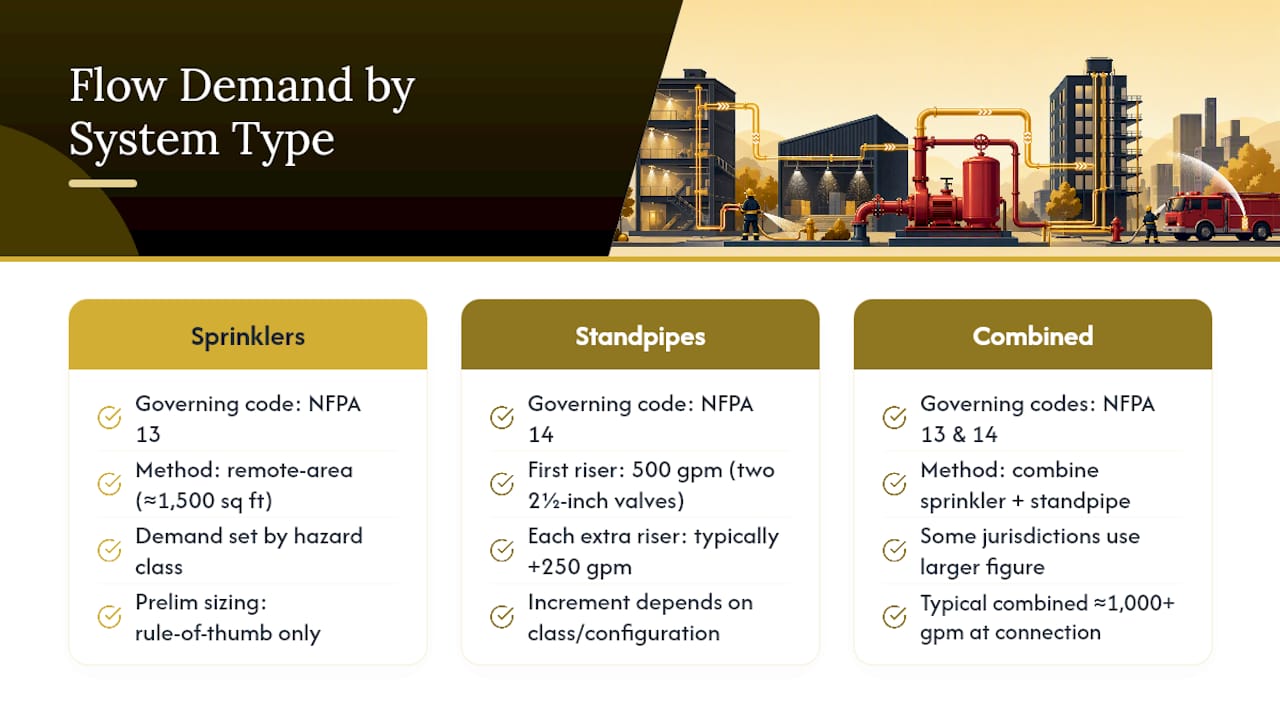
For sprinkler systems, NFPA 13 governs the remote-area method, which models the worst-case zone, typically 1,500 square feet, based on the hazard classification of the occupancy. Light hazard occupancies demand less water per square foot than ordinary or extra hazard spaces, so the classification you assign at the start of a project quietly controls everything downstream.
Standpipe systems follow a different logic entirely, laid out under NFPA 14. The first standpipe riser requires 500 gpm delivered to the two most remote 2½-inch hose valves. Each additional riser typically adds 250 gpm to total system demand, though the specific increment depends on the standpipe class and building configuration.
Combined systems, where sprinklers and standpipes share the same water supply, require you to add the sprinkler demand to the standpipe demand, or in some jurisdictions use the larger of the two figures rather than a strict sum. Sizing a fire pump means calculating flow and pressure together under both NFPA 13 and NFPA 14 rules, and most combined systems land somewhere between one thousand and slightly above that range at the point of connection, though local code amendments can push that cap in either direction.
During preliminary sizing, experienced engineers often rough out demand using rule-of-thumb figures for the occupancy type before committing to a full hydraulic model. That shortcut works for early budget conversations. It does not work for a stamped drawing, and any number you use for procurement or permitting has to come from a full remote-area or standpipe calculation, not a back-of-envelope estimate.
Converting Flow Demand Into Required Pump Discharge Pressure
Once you know the flow rate, the next question is pressure, and this is where the formula from the top of this article gets applied line by line.
Total pump discharge pressure equals static head, in psi, plus required residual pressure, in psi, plus friction loss, in psi. Static head comes from elevation. Every foot of vertical rise between your reference point and the highest or most remote outlet costs you 0.433 psi. A building with 120 feet of elevation difference between the pump and its top-floor sprinkler head carries a static head requirement of roughly 52 psi, calculated as 120 multiplied by 0.433.
Residual pressure is the minimum pressure your code requires at the most remote hose connection or sprinkler head once water is actually flowing. Standpipe systems commonly require residual pressure in the mid-60s to about 100 psi range at the topmost outlet, depending on jurisdiction and application. Always verify the applicable figure against the governing code edition and any local amendments rather than assuming a national default applies everywhere.
Friction loss, the third term, gets its own full treatment in the next section, but it belongs in the same sum: static head, residual, and friction loss all add together to produce the number the pump has to overcome.
- Static head: elevation difference in feet multiplied by 0.433 psi per foot
- Required residual: code minimum at the most remote outlet, commonly 65 to 100 psi
- Friction loss: cumulative pressure drop through pipe and fittings at design flow
- Safety buffer: engineers frequently add 20 to 50 psi to account for supply fluctuations in the municipal main
That last point matters more than it looks. Municipal water pressure isn't static. It shifts with time of day, seasonal demand, and nearby construction. Building in a buffer isn't padding for its own sake, it's insurance against a supply curve that moves after your design is locked.
How Friction Loss Gets Calculated Through the Pipe Network
Friction loss is where most of the actual arithmetic in a hydraulic calculation happens, and the Hazen-Williams equation is the tool nearly every fire protection engineer reaches for to do it. It's an empirical relationship between flow rate, pipe diameter, pipe length, and a roughness coefficient known as the C-factor, and it has dominated fire protection hydraulics for decades because it's accurate enough for the pressures and velocities typical of sprinkler and standpipe systems.
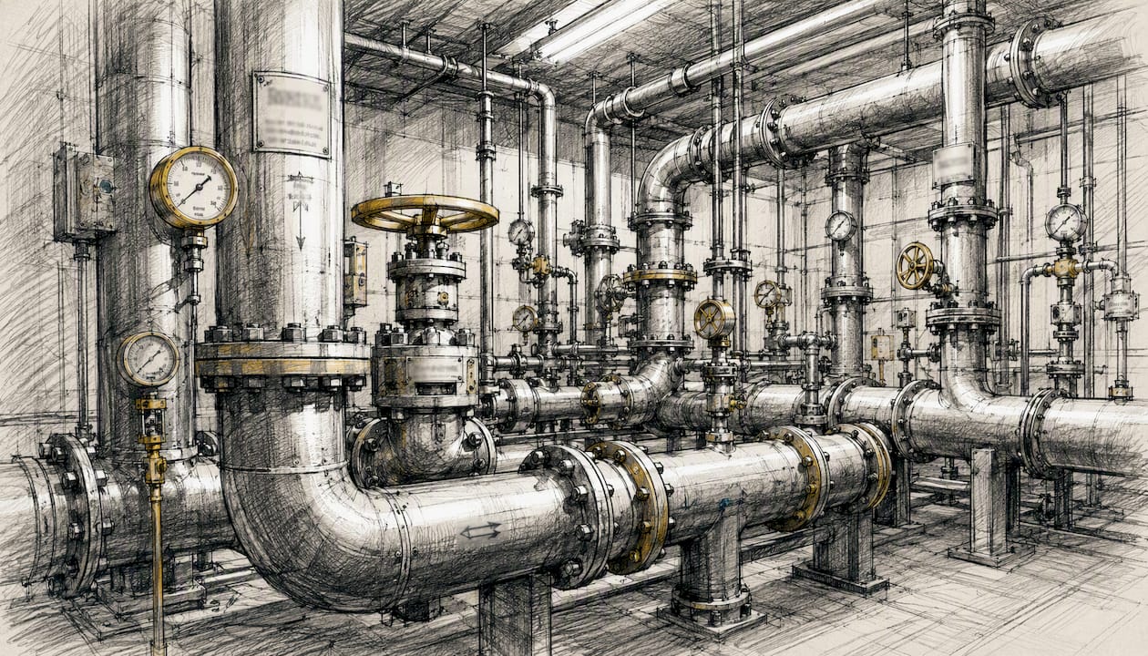
The C-factor you select depends on pipe material and, critically, age. New steel pipe carries a different roughness coefficient than pipe that's been in service for twenty years and accumulated internal scale. NFPA 13 provides standard C-factor tables for common materials, and using an optimistic factor for aged pipe is one of the more common ways a friction-loss calculation understates real-world pressure drop.
Fittings add loss too, and you can't calculate them the same way you calculate straight pipe. Instead, every elbow, tee, and valve gets converted to an equivalent length, meaning the length of straight pipe that would produce the same friction loss as that fitting. Add those equivalent lengths to your actual pipe run before running the Hazen-Williams calculation, and you get a realistic total.
Velocity pressure, a separate term that accounts for the kinetic energy of moving water, typically gets omitted in fire protection calculations because it's small relative to friction loss and static head, and omitting it produces a slightly conservative, safer result. Most engineers skip it for that reason unless a specific code provision or unusual system geometry calls for it.
For actual number-crunching, friction-loss tables derived from Hazen-Williams remain a standard field reference, and pairing them with a spreadsheet or hydraulic calculation program keeps units consistent from one pipe segment to the next. Whatever method you use, manual table or software, verify that every input carries the same units before trusting the output.
Using K-Factors to Calculate Sprinkler and Nozzle Flow
Every sprinkler head and hose nozzle has a K-factor, and that single number is what links the pressure at the device to the flow rate coming out of it.
The relationship is straightforward: Q equals K multiplied by the square root of P, where Q is flow in gpm, K is the device's orifice coefficient, and P is pressure in psi at the device. A sprinkler with a K-factor of 5.6 operating at 20 psi discharges roughly 25 gpm, since 5.6 times the square root of 20 works out close to that figure. Change the pressure and the flow changes with it, but not linearly, which is why pressure swings at the far end of a system have an outsized effect on total demand.
- Locate the K-factor on the manufacturer's data sheet or the sprinkler's nameplate, since every listed device carries a documented, tested value.
- Apply it in the model at the pressure the hydraulic calculation predicts at that specific device, not at the pump discharge.
- Cross-check with a pitot tube during hydrant or hose-stream testing by reading the pitot pressure and converting it to flow using the same orifice relationship, now solving for Q from a known nozzle coefficient and measured P.
- Use pitot readings for acceptance testing, comparing the calculated flow against the pump's nameplate rating to confirm the system performs as designed once it's installed.
Pitot tube testing isn't just a field verification exercise, it's the same math running in reverse. Instead of predicting flow from a design pressure, you're measuring actual pressure at a nozzle and backing into actual flow, which is exactly how acceptance tests confirm a system performs the way the calculation said it would.
Reading a Hydrant Flow Test and Plotting the Supply Curve
A hydrant flow test gives you data points including static pressure and residual pressure at a measured flow, and from those points you build the water-supply curve that every downstream pump decision depends on.
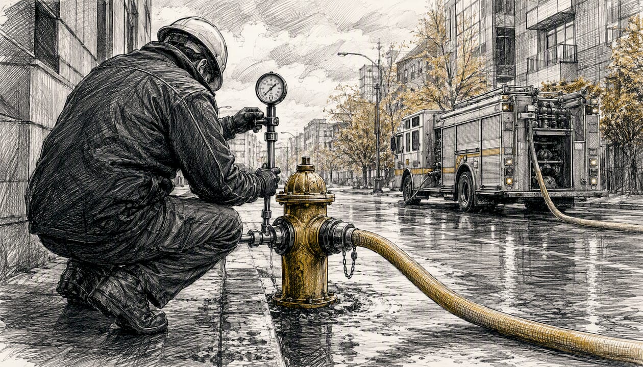
The test procedure itself is straightforward on paper. Open a flow hydrant and measure the resulting flow rate with a pitot gauge or calibrated diffuser, while simultaneously reading residual pressure at a nearby test hydrant that's closed and gauged. Record the static pressure before any flow starts. Document the date, the hydrants used, and their distance from the point where the water actually enters the building, because that distance affects how representative the test is of real supply conditions at the riser.
Plotting the curve is simple algebra once you have the two points: static pressure at zero flow, and residual pressure at the tested flow rate, connected by a curve that follows a known hydraulic relationship. Overlay the system demand curve, built from the flow-and-pressure requirements calculated in the previous sections, on the same chart. Where the demand curve sits below the supply curve at the design flow, the municipal supply alone is adequate. Where demand exceeds supply at that flow rate, a fire pump becomes mandatory to make up the difference.
Pro Tip: Test as close to the building's point of connection as the water utility will allow. A hydrant two blocks away with different main sizing or a different pressure zone can show a supply curve that has nothing to do with what actually reaches your riser.
Selecting a Pump and Validating the Duty Point on the Curve
With demand and supply both established, pump selection becomes a matter of finding the pressure gap and choosing hardware that closes it without violating NFPA 20's acceptance criteria.
NFPA 20 requires the pump's performance curve to intersect the system demand somewhere between 100% and 150% of the pump's rated flow, and it sets three specific test points every pump must satisfy: churn pressure at zero flow cannot exceed 140% of rated pressure, the pump must deliver 100% of rated flow at 100% of rated head, and at 150% of rated flow, pressure cannot fall below 65% of rated head. Those three constraints define the shape every acceptable pump curve has to follow.
- Calculate the pressure boost required, the difference between what the system demands and what the water supply curve delivers at the design flow.
- Divide the system demand by 150% to find the minimum rated flow a standard pump size needs to carry, then round up to the next available standard pump rating.
- Plot the candidate pump's curve against the demand curve and confirm the intersection point falls within the 100% to 150% range, not right at either edge.
- Check the churn pressure against downstream component ratings, and flag any pump whose zero-flow pressure would push system pressure past a 400 psi hose valve limit.
- Apply the affinity laws if you're adjusting an existing pump's speed or trimming its impeller, since flow scales linearly with speed while head scales with the square of speed, and power scales with the cube.
Some engineers push the design point toward 150% for the smallest possible pump, but targeting a design point between 115% and 135% of rated flow instead of right at the ceiling gives you margin against future changes to the building or the water supply. Driver sizing follows a similar logic: motors typically carry roughly a 15% margin over calculated shaft power so the motor isn't overloaded at the 150% overload point, where power draw peaks even as pressure drops.
Verifying Suction Conditions to Avoid Pump Cavitation
Everything so far has dealt with the discharge side of the pump. The suction side gets less attention and causes more field failures, because a pump that can't get enough water into its eye will cavitate regardless of how well the discharge side was calculated.
Net Positive Suction Head Available, or NPSHa, is built from four components: the static suction head, atmospheric pressure at the site, the vapor pressure of the water at its operating temperature, and the friction losses through the suction piping, adjusted for elevation. NPSHa must exceed the manufacturer's published NPSHr, the required value at the pump's rated flow, and the margin between them isn't a nicety, it's the difference between smooth operation and a pump that cavitates the first time it runs at full demand.
Cavitation shows up as noise that sounds like gravel running through the casing, a drop in discharge pressure that doesn't match the flow being demanded, and over time, physical pitting on the impeller vanes that shortens pump life dramatically. NPSHa must strictly exceed NPSHr at every flow condition the pump will actually see, not just at its rated point.
On the piping side, keep a minimum straight run of suction pipe upstream of the pump inlet, install eccentric reducers with the flat side up to avoid trapping air, and size the suction pipe to NFPA's minimum diameter recommendations for the pump's rated flow. Skipping any of these details tends to produce a system that runs fine on paper and cavitates the first week it's in service.
Worked Example: From Hydrant Test to Pump Selection
Here's a complete calculation from raw hydrant numbers to a final duty point, with every unit accounted for along the way.
Start with hydrant flow test data: static pressure and residual pressure at a known flow rate. That gives you the two points needed to build the supply curve.
System demand: assume a combined sprinkler and standpipe system requiring 1,100 gpm at the point of connection, based on a remote-area sprinkler calculation of 600 gpm combined with a single standpipe riser demand of 500 gpm. Elevation from the pump room to the highest standpipe outlet is 140 feet, giving a static head of 140 multiplied by 0.433, or roughly 61 psi. Friction loss through the piping network at 1,100 gpm, calculated via Hazen-Williams across the full run including fitting equivalent lengths, comes to 48 psi. Required residual pressure at the topmost hose valve is set according to applicable standpipe code provisions, often around 100 psi.
- Sum the pressure components: 61 psi static head, plus 100 psi required residual, plus 48 psi friction loss, equals 209 psi total required discharge pressure at 1,100 gpm.
- Compare against supply: at 1,100 gpm, the hydrant supply curve (built from the 78 psi static and 52 psi at 1,000 gpm points) delivers roughly 47 psi, well short of the 209 psi demanded, confirming a fire pump is required.
- Calculate the boost needed: 209 psi minus 47 psi leaves a required pump boost of approximately 162 psi at 1,100 gpm.
- Divide demand by 150%: 1,100 divided by 1.5 equals about 733 gpm, so the minimum standard pump rating to consider starts around 750 gpm, though a 1,000 gpm rated pump is a common standard size that gives more margin.
- Validate on the curve: a 1,000 gpm pump rated at 165 psi would put the 1,100 gpm demand point at 110% of rated flow, comfortably inside the 100% to 150% window, with churn pressure checked against the 140% limit (231 psi maximum) and the hose valve's 400 psi ceiling.
| Calculation step | Value |
|---|---|
| System demand flow | 1,100 gpm |
| Static head (140 ft × 0.433) | 61 psi |
| Friction loss at design flow | 48 psi |
| Required residual pressure | 100 psi |
| Total required discharge pressure | 209 psi |
| Selected pump rating | 1,000 gpm at 165 psi |
| Duty point as % of rated flow | within NFPA 20 required range |
Round pressure figures to the nearest whole psi and flow figures to the nearest 50 gpm for reporting purposes, since false precision beyond that doesn't reflect the accuracy of the underlying hydrant and friction-loss data.
Choosing Between Software Tools and Manual Verification
Hydraulic analysis software has replaced hand calculation for most production work, but the tools only produce a reliable duty point when the person running them understands what the output should look like before the program tells them.
Full network hydraulic analysis packages, sometimes referred to under names like HASS, solve complex piping networks with dozens of nodes simultaneously, something that would take hours by hand. Pump manufacturers also publish curve-selection tools tied to their own product lines, and field crews rely on handheld calculators, including Task Force Tips (TFT) devices, for quick nozzle flow and pressure conversions during hydrant testing and hose-stream evaluation.
The right workflow uses software for the iterative network solve, the part that's tedious and error-prone by hand, while reserving manual checks for the handful of numbers that matter most: where the duty point lands on the pump curve, whether NPSHa clears NPSHr with margin, and how the hydrant supply curve compares to system demand. Those three checks take minutes to verify by hand and catch a meaningful share of the errors that slip through automated models.
Manual verification isn't optional at certain points in a project. Acceptance testing, quality control review, and any witness test with the authority having jurisdiction present all require someone to confirm the numbers independently of whatever software generated the original design. Software is only as good as what goes into it, so double-check hydrant test inputs and device K-factors before trusting an automated output, since a wrong K-factor entered once can silently propagate through an entire model.
Verification Checklist and Common Calculation Mistakes
Before any calculation goes into a submittal package or an equipment order, run it against a short list of checks that catch the errors most likely to slip through.
- Confirm every input, hydrant data, elevations, pipe sizes, is current and matches the actual as-built conditions
- Verify unit consistency throughout, especially the feet-to-psi conversion at 0.433 psi per foot
- Plot supply against demand and confirm the pump closes the actual gap, not an assumed one
- Check NPSHa against NPSHr with margin at the pump's full operating range, not just the rated point
- Confirm the pump curve intersects demand between 100% and 150% of rated flow
- Verify churn pressure doesn't exceed downstream component ratings, particularly the 400 psi hose valve limit
- Confirm the design is ready for a witnessed acceptance test with documented churn, rated, and overload readings
The mistakes that show up most often in field reviews follow a pattern. Outdated hydrant data tops the list, followed closely by unit conversion errors between feet and psi that go unnoticed until a pressure reading doesn't match expectations. Forgetting fitting equivalent lengths understates friction loss. Misapplied K-factors, often a nameplate value swapped for a similar-looking model, throw off flow predictions. Exceeding the 400 psi hose valve limit at churn is a completed-design problem that should never survive a proper check. And neglecting suction-side losses produces a pump that looks perfect on the discharge side and cavitates the moment it starts.
A recommended commissioning sequence runs the pump at churn first, records the reading, opens to rated flow and records again, then opens further to the 150% overload point and records a third time, all within about 5% of nameplate values and witnessed by the AHJ or the owner's representative using calibrated flow-measurement equipment.
What Bazini Engineering Has Learned From Hydraulic Calculations in the Field
The single biggest lever on accuracy in this entire process is where you choose to test. A hydrant test performed at the actual point of connection to the building, rather than at the nearest convenient hydrant, removes an entire category of uncertainty from the rest of the calculation. When that's not possible, the right move is a conservative buffer, typically in the 20 to 50 psi range, applied to account for supply fluctuations rather than assuming the tested condition holds every day of the year.
Documentation matters as much as the math. Every assumption, the hazard classification used for remote-area sizing, the C-factor applied to aged pipe, the safety margin built into the pressure calculation, belongs in the final report where a reviewing engineer or the AHJ can see exactly what was assumed and why. A calculation without documented assumptions is a black box, and black boxes don't survive plan review.
Coordination with the water utility early in a project, before the hydraulic model is finalized, often changes the outcome. Utilities can flag main upgrades, pressure zone boundaries, or known supply limitations that aren't obvious from a single flow test. Combine that with witnessed acceptance testing per NFPA 20, where churn, rated, and overload points get documented against nameplate values, and the design has been checked twice: once on paper, once in the field.
Pro Tip: Build your pressure buffer around what the water utility tells you about seasonal or peak-hour demand, not just what a single flow test on a single afternoon happened to show.
Why the Same Steps Play Out Differently on Every Project
We approach every fire pump calculation the same way on paper, gather hydrant data, calculate demand, compute friction loss, validate against the pump curve, but the actual sequence of decisions rarely looks identical from one project to the next. A retrofit in an existing building with aged piping demands a much harder look at the C-factor assumption than new construction, because the roughness inside twenty-year-old steel pipe can shift friction loss enough to change which standard pump size actually clears the acceptance points.
Coordination with the local water utility and the authority having jurisdiction shapes the final design more than most first-year calculations account for. A utility that flags a planned main upgrade, or an AHJ with a local amendment on residual pressure requirements, can move the target pressure enough to change the pump selection entirely, which is why we treat those conversations as part of the calculation process rather than a formality that happens after the numbers are locked.
How Bazini Engineering Supports Your Fire Pump Project
Getting from a hydrant test to a stamped pump selection involves a lot of steps where a small error compounds, and that's exactly the work Baziniengineering handles for building owners, architects, and contractors who need a hydraulic calculation they can submit with confidence.

A typical fire pump engagement with Baziniengineering includes coordination of the hydrant flow test itself, a complete hydraulic calculation report covering demand, friction loss, and required discharge pressure, pump-curve plotting with documented validation against NFPA 20 acceptance points, NPSHa verification against the selected pump's suction requirements, and acceptance-test support when the pump is commissioned as part of comprehensive fire alarm systems and life safety integration. What you get at the end isn't just a number, it's a full report with calculations, supply and demand curve plots, and test records that stand up to plan review and AHJ scrutiny. For buildings where pump room mechanical coordination or broader plumbing scope factors into the installation, Baziniengineering's mechanical engineering and plumbing engineering teams work alongside the fire protection group so the pump room design accounts for everything around it, not just the pump itself.
If you're planning a new fire pump installation, evaluating an existing one, or need a hydraulic calculation report for permit submittal, reach out through Baziniengineering's fire suppression services page to request a project quote.
Standards and Tools Worth Consulting
Every hydraulic calculation ultimately traces back to a small set of governing standards and reference tools, and knowing which one answers which question saves time on every project.
NFPA 13 governs sprinkler system design and remote-area demand calculations. NFPA 14 sets standpipe flow and pressure minimums. NFPA 20 controls fire pump selection, installation, and the acceptance testing that confirms a pump performs as designed. Beyond the standards themselves, Hazen-Williams friction-loss references and tables remain the standard method for calculating pipe losses, and orifice or K-factor references from sprinkler and nozzle manufacturers provide the device-specific data every model depends on. In the field, tools like TFT calculators handle quick pitot-to-flow conversions, while full hydraulic analysis software handles the network-wide solve for complex systems.
Local code amendments and individual water utility requirements can shift specific numbers, residual pressure minimums, flow caps, testing protocols, so always confirm the current edition adopted in your jurisdiction and check directly with the water utility before finalizing a design based on general guidance alone.